
iVaR - Frequently asked questions
Find the answer to your most pressing questions regarding iVaR.
What is iVaR?
Traditional investment risk measures that are still used today, such as volatility, have historically been chosen because of their simple mathematical properties. They do not work well to describe the risk of real investment portfolios and are not consistent with what end investors perceive as risk.
Following the above observations, we developed a new, innovative risk measure which we call InvestSuite Value at Risk (iVaR). Our basic premise is that any instrument or portfolio providing strict monotonic growth (i.e., no losses) should be riskless, regardless of the speed or consistency of the growth. The reason for this premise is that it matches the behaviour of a savings account, which also increases monotonically in value over time, and is considered riskless by end investors. For instruments or portfolios that do not exhibit monotonic growth (i.e. the vast majority) we calculate the risk (“iVaR”) as the deviation from monotonic growth.
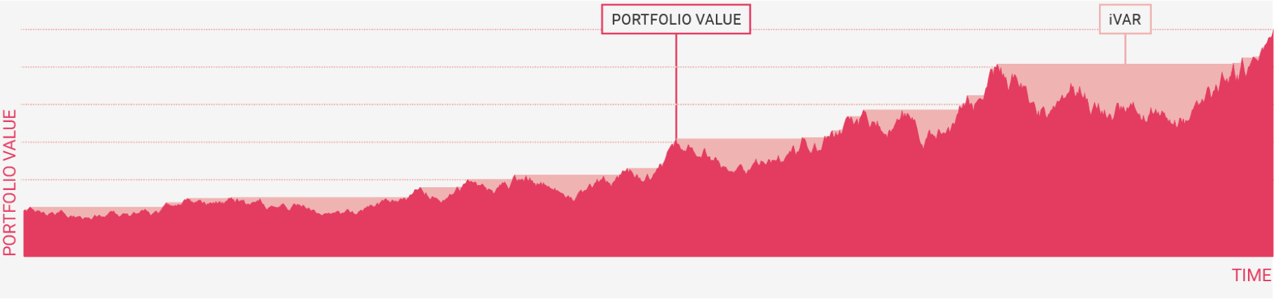
In practice, this deviation is calculated as the difference between the actual value at each point in time and the highest value ever seen up to that point in time. The difference between the two is visualised as the sum of the pink areas.
The difference between the two, the sum of the pink areas, is our measure for investment risk, called iVaR (InvestSuite Value at Risk). It is a combination of the size of losses (the height of the pink areas) and the time it takes to make up for those losses (the width of the pink areas). This 4th generation human centric measure of risk can also be used to define relative risk versus a benchmark, similar to how volatility can be used to define relative risk via tracking error.
Using this risk measure in portfolio construction should lead to portfolios that suffer lower losses (versus a benchmark) and make up for those losses more quickly, compared to traditional risk measures.
What is the difference between iVaR and other traditional measures of risk?
Our white paper: “The human-centred, next-generation quantitative approach to constructing portfolios” explains the differences between iVaR, conditional Value-at-Risk, Value at Risk and volatility in depth. On the graph below we indicate the major differences between those measures of risk. A key feature of iVaR is that it takes into account the total joint return distribution of all assets in the investment universe, making it a 4th generation measure of risk.
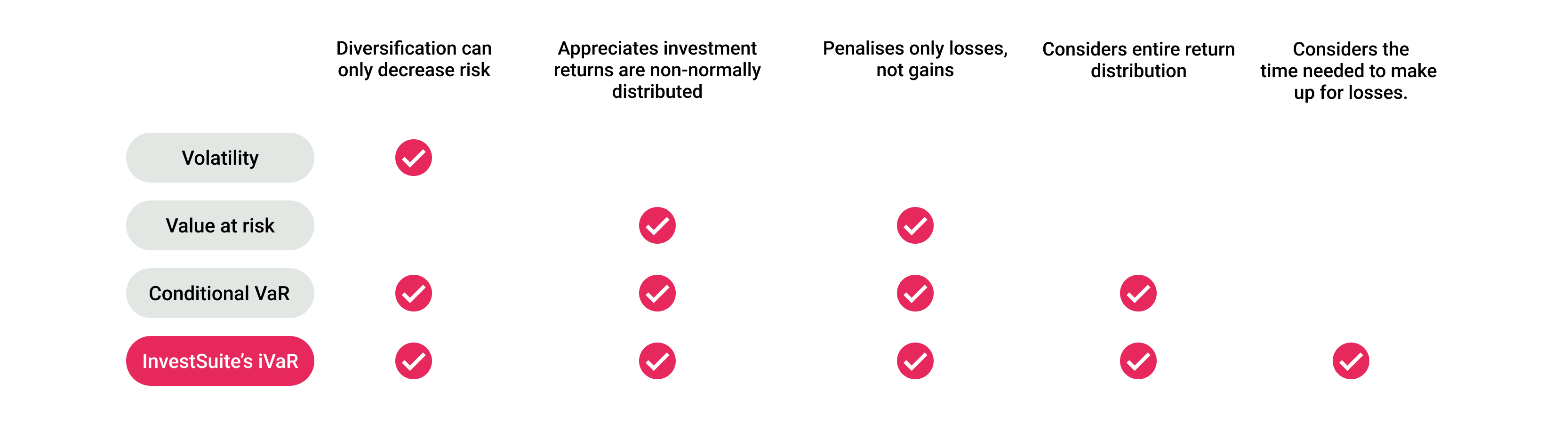 4th GENERATION RISK MEASURE - iVAR ADDRESSES THE SHORTCOMINGS OF VOLATILITY, VAR AND CVAR
 What is so different about InvestSuite’s approach compared to traditional investment managers?
The philosophy behind what we do is very different from that of most investment managers. We have a very strong focus on minimising drawdowns in 3 aspects: frequency of the drawdowns, size of the drawdowns and the time to recover.
Therefore, we think our iVaR philosophy is more consistent with what end investors actually care about.
Which instrument types can be used in the portfolio construction?
The universe can consist of a broad range of instrument types, e.g. stocks, bonds, ETFs, Mutual Funds, cryptocurrencies, etc.
Instrument types with highly skewed distributions such as structured products can be supported as well. In the latter case the only requirement for an instrument to be incorporated in the universe, is to have sufficient (reconstructed) historical time series data.
How many instruments should be in the investment universe and how diverse (uncorrelated) do the underlying instruments have to be?
Irrespective of the risk measure that is used within the portfolio construction, it is important for the Portfolio Optimizer to have sufficient diversification options. This is, however, very hard to quantify. For any hypothetical investment universe, InvestSuite can check the “diversification ratio”, i.e. comparing the risk of the portfolio to the weighted average of the risks of the individual investments. This can give a good indication of whether the investment universe is diversified enough.
Did you backtest your algorithm? What are the results?
We did a proper ”point in time” backtest of our algorithm using data going back to the late 1990’s (this is actually not that easy as ETFs did not exist back then, so we had to use data for the indices underlying the ETFs and subtract costs). When running the backtest, at the end of each month we fed data available up to that point to our portfolio construction algorithm, rebalanced the portfolio and held it constant until the end of the next month.
Not only do the backtests show that we would have achieved our key objective (minimising deviation from expected monotonic growth) very well in practice, they also show that the approach of limiting that risk would not have resulted in a lower return. Of course it is important to note that past performance may not be indicative of future performance.
We also run “live” backtests which are updated daily for different “academic” or “paper” portfolios.
What is the time horizon for which the iVaR based optimisation is best suited?
The iVaR based optimisation is calibrated to minimise the risk (as defined by iVaR) in the near future. There is no real point in trying to minimise the risk further in the future, as our methodology is inherently dynamic and can rebalance as time goes on and market circumstances change. This constitutes a major difference in comparison to classical risk management applications that try to predict longer term risks when holding illiquid instruments.
If your approach is so wonderful, then why are the largest asset managers of the world not doing this?
The philosophy behind what we do is very different from that of most investment managers.
In managing risk, they generally look at tracking error compared to a reference benchmark. Their performance is usually evaluated based on the information ratio versus this benchmark. We think our iVaR philosophy is more consistent with what end investors actually care about. Portfolio Optimizer is a portfolio construction framework that allows traditional investment managers to combine their views on the markets and restrictions with a 4th generation human centric risk framework.
Why not the classic model portfolios?
Classic model portfolios are usually simple market cap weighted portfolios. They hold all countries, sectors, stocks, etc. proportional to their size (in terms of market capitalization). The reason for doing this is that they assume market cap weighted portfolio are risk-return efficient, which research has repeatedly shown they are not (see for example Haugen & Baker, Journal of Portfolio Management, 1991).
Classic model portfolios for different risk profiles usually have the same compositions for their equity and fixed income parts, and equity vs fixed income weight just varies between risk profiles. This is again not risk-return efficient: a more defensive investor should for example hold more defensive equity than a dynamic investor.
Classic model portfolios assume investors are all identical and have no personal preferences. We believe some investors may for example want to invest in a socially responsible way or exclude certain investments (e.g. emerging markets). This more customised approach is not compatible with classic model portfolios.
Model portfolios cannot be “backtested”: we cannot simulate what a model portfolio’s performance would have been before its inception because we cannot go back in time and ask what the model portfolio’s investment committee would have proposed to invest in (unless the model portfolio’s investment strategy is simple enough that it can be automated without an investment committee). Our portfolio construction method can be asked what advice it would have produced in the past with the data that was available at that time, and therefore can be backtested.
How much returns do you give up by minimising the “risk”?
Fundamentally, risk and return are different concepts, and therefore we cannot fully minimise one while simultaneously fully maximising the other. Therefore, there must be a trade-off between risk and return and we must give up some return if we only focus on minimising risk.
Classic financial theory predicts that risk and excess return should be proportional to each other and taking higher risk should therefore result in a proportionally higher return. This is a strong statement because it means that minimising risk implies a simultaneous decrease of the returns.
However, the low volatility anomaly shows that in practice, the trade-off between risk and return is not as bad as the above relationship. On the contrary: in most markets, low volatility stocks have historically achieved higher returns than high volatility stocks.
A second effect is called volatility drag. The result of this is that you can achieve a higher compounded portfolio return over time by lowering volatility by itself. So it is not necessary to achieve a higher median or even arithmetic mean average return to be able to provide compounded outperformance.
The result of this is that, at least historically, it has been perfectly possible to decrease risk without necessarily decreasing returns. We of course can’t guarantee that the low volatility anomaly will hold in the future.
At the moment, we force a minimum allocation to equity, ensuring enough exposure to higher return-generating assets. In the future, we will work with setting minimums on market implied expected returns rather than just focus on minimising risks.
How do you handle currency risk if you are in a non EUR / USD country?
We prefer to optimise portfolios (i.e. minimise their risk) in the currency of the investor, as risk can differ depending on which currency you calculate the risk in
For example, if USD drops 10% compared to the Euro, this will not impact a USD investor, but it will of course impact an Euro investor that invests in securities that have exposure to USD. Since our portfolio construction method minimises risk in the investor’s currency, it will for example complement USD-based investments with others so that the EURO-denominated value has minimal risk.
However, the built-in currency hedging of the previous point does not work well for fixed income ETFs. For currencies such as GBP/CHF/JPY there are sufficient ETFs that invest in local currency fixed income ETFs, such that currency risk can be avoided.
For other currency investors, currency hedging could be an option, or we could widen the investment universe to include regular funds, which more often exist in local market or currency hedged versions
For equity, the problem is not that big, as currency risk is generally much smaller than equity risk. Also, due to the fact that local equity market returns and currency returns tend to be negatively correlated, having some currency exposure is often actually risk reducing.
How do you make sure to be protected against drawdowns in the future, when markets may behave totally differently from today?
The iVaR approach is dynamic and takes into account current market circumstances. This means that, if markets start behaving totally differently over time (as they often do), the iVaR methodology will pick up on this changing behaviour and reallocate the portfolio accordingly. In short, when minimising for iVaR the proposed portfolio will shift out of assets with a high sensitivity to systemic risk at that point in time. As an example, in 2005 financial stocks did not behave yet as being very sensitive to risk on/off sentiment, but by end 2006 they started to, and the non-relative iVaR methodology therefore shifted out of financials long before the actual 2008 financial crisis.
Which quality measures/macro data do you use in the algorithm?
At the moment, we do not explicitly take into account quality or macro-economic data. We of course implicitly take them into account:
- Lower quality investments will tend to exhibit more volatility, leading our algorithm to avoid them;
- Macro data is also immediately reflected in the price of investments and therefore taken into account by our algorithm. We do not believe in predicting macro variables ourselves (research has repeatedly shown this is near impossible), but what we will be working on next year is on modelling probabilities of where we are in the business cycle and optimising portfolios while taking that into account.
Can you take our views into account?
Yes, at the moment we already allow our clients to incorporate their views in one of 2 ways:
- either they set minima/maxima on the exposure to certain parts of the market (asset classes, regions, sectors, bond types, etc…),
- or they can define their expected returns for each investment and we can minimise portfolio risk (according to our iVaR metric) subject to achieving at least a certain expected return (or vice versa, maximising expected return subject to a maximum risk level).
Does Portfolio Optimizer or iVaR involve AI or Machine Learning?
This all depends on what is considered to be AI/Machine Learning. Yes, Portfolio Optimizer does learn from past investment price data to find the optimal portfolio that limits future investment risk within the given constraints. Yes, here at InvestSuite, we are developing GARCH/DCC models that are able to learn from historical data how market dynamics tend to behave and turn that into realistic simulation of scenarios that describes how the future could look like.
No, Portfolio Optimizer does not use “generic” AI such as neural networks. The simple reason for this is that there is not enough independent data to train these generic algorithms on, and the market dynamics change so quickly over time that a model trained to a specific period would break down in the next period. Therefore in investment analysis, these generic models are not often used.
To give an example comparison: it is straightforward to find millions of pictures of cats. Hence, it is relatively easy to train a neural network to recognise a cat. In the last 20 years, however, there have only been a couple of independent recessions, so there is very little data to train a neural network on what a recession looks like. Furthermore, the world is in a totally different place than 20 years ago, so the things that may have caused a recession then may have become irrelevant today. On the other hand, a cat from 20 years ago still looks like a cat.
Because of this lack of “unlimited” data, models that work well in investment management usually have some structural form that is imposed, such that the number of parameters that need to be learned by the model is not too excessive and can be trained with a more limited data set without risking too much overfitting.
Where did you get that Markowitz quote? It doesn’t sound correct to me!
Over the last decades, Markowitz has repeatedly admitted that the assumptions behind Modern Portfolio Theory (MPT) & the capital asset pricing model (CAPM) are flawed and that the conclusions of MPT/CAPM do not hold empirically. Below are a few quotes from Markowitz that come from this 2017 interview with Andrew Lo from MIT and his 2005 paper “Market Efficiency: A Theoretical Distinction and so What?”
- “A lot has happened since I published that article in 1952. Now there’s infrastructure, we have data that goes back to 1926 at least. [...] Now we have optimisers, we didn’t have an optimiser in 1952.”
- “I don’t know about you, but I can’t borrow all I want at the risk free rate. Due to investors not being able to borrow at the risk free rate, I don’t believe that the market portfolio even is an efficient portfolio. And it is certainly not an efficient portfolio for everybody.”
- “It is true that there is no linear relationship between expected return and beta (market sensitivity).”
- “The correct portfolio for the individual depends on risk preferences. There are constraints on the choice of portfolio which varies from individual to individual, they have shorter or longer horizons, they are willing to invest in certain asset classes or not, they have different tax situations etc. There is no perfect portfolio, but there is a right portfolio for a specific individual, but it’s a lot of work to find them. Part of the process is always to involve the investor.”
It is quite paradoxical that a lot of robo advisors that proudly claim to be based on Markowitz’s “nobel prize winning technology” ignore the insights Markowitz himself gained over the last 65 years. Which, for example, is that the market portfolio is not an efficient portfolio, that taking on higher market sensitivity is not always rewarded by higher expected returns and that portfolio optimisation should be highly personalised. Our investment approach is consistent with Markowitz’s 2017 views on how to construct an investment portfolio, not his 1952 views.
Why are individual, or hyper-personalised, portfolios better than model portfolios?
Investors have different time horizons, risk tolerances, tax situations, risk exposures (e.g. through their job or holdings in private companies), which should by itself already result in a different investment portfolio for each client. But Harry Markowitz makes a great point in this 2017 interview when he says that it is crucial that investors invest in a portfolio that is invested in assets they feel comfortable with. Retail investors massively lose out on performance - about 3% per year(!) - by buying and selling their risky investments at the wrong point in time. If an investor is not fully comfortable with an investment portfolio, the probability of him selling out of it during a time of crisis is much higher. This can be solved with a more personalised portfolio, which is exactly what our approach aims to achieve. And of course a personalised portfolio provides a much better user experience than forcing investors into a plain vanilla standardised product
Individualised portfolios also allow our direct clients (the banks/brokers) to incorporate their views into the portfolios, something they wouldn’t be able to do if we forced them to use a set of model portfolios that we decided on.
How do you take into account the risk profile? How do you use the SRI scores?
There is no strict regulatory definition of what a risk profile should entail, so the client can define what (s)he means with a certain risk profile (e.g. maximum exposure to equity, maximum SRI score in the universe, maximum weighted average SRI score of the portfolio, …). We should be able to fully support the way the client defines its risk profiles.
For our backtests, we used the simplest possible way of defining risk profiles: setting the percentage equity to a fixed value (0/25/50/75/100%).
How far back in time does the data set need to go to allow the algorithm to calculate iVaR? Is there a minimum length of time and then perhaps an ideal length of time?
We need at least 3 years of historical data for all instruments. This doesn’t mean that all instruments have to exist for 3 years, we have ways of using proxies (i.e. underlying index of a fund/etf) or modelling historical returns based on factor models.
What is your rebalancing methodology?
The rebalancing frequency and criteria can be fully customised by our B2B client. What we propose is to not set a fixed rebalancing frequency, but rather make it dynamic and propose a balancing when a sufficient expected reduction in iVaR can be realised.
Which data are used within Portfolio Optimizer and for iVaR?
When Portfolio Optimizer is only used to minimise the risk in the portfolio, it solely requires historical time series data. When additional restrictions, e.g. sectoral or regional limits, are applied, additional data is of course needed. We have data contracts with some of the main data providers. Alternatively, our Portfolio Optimizer can be run with custom data from our clients.
Can I use the Portfolio Optimizer to construct individual portfolios with iVaR for every single retail client?
Yes. Portfolio Optimizer is a cloud-based optimisation tool that is built to allow customisation at scale. Therefore, it is extremely well suited to create hyper-personalised portfolios for retail clients. Our B2B clients can, of course, determine the degree of personalisation that is allowed for each end client.
Nevertheless, the Portfolio Construction algorithm will take into account all available data up to that point in time. Two similar retail clients with exactly the same setup can have slightly different proposed portfolios depending on the date on which the proposed portfolio is being constructed.
How can we differentiate if you sell the same product to a competitor?
Our Portfolio Optimizer is a cloud-based portfolio construction tool that is built to allow customisation at scale. Among others, our clients can:
- Select a custom investment universe
- Define a customised objective consisting of among others minimising risk, minimising relative risk, maximising ESG scores etc.
- Implement a custom investment policy that can include in-house views on asset class, sector, region, bond type, etc.
- Set minima/maxima on the exposure to certain parts of the market (asset classes, regions, sectors, bond types, etc.). Those limits can also be set relative to a benchmark.
- Optionally define expected returns for each investment. Our Portfolio Optimizer can minimise portfolio risk subject to achieving at least a certain level of expected return (or vice versa, maximising expected return subject to a maximum risk level)
- Use a custom rebalancing logic/frequency
- Use a custom client user interface.
In general, we aim at having bank level parameterisation possibilities that are very exhaustive. More information can be found in our API documentation.
Glossary
Drawdown
A drawdown is the peak-to-trough decline of an investment during a specific recorded period. A drawdown is usually quoted as the percentage between the peak and the subsequent trough.
Volatility
Mathematically, it is calculated as the standard deviation of the returns of an investable asset. It is therefore a measure for “absolute risk” and indicates how likely the performance of an investment is to significantly deviate from the return of a cash investment. Usually, annualised numbers are used. A tracking error of 16% means that (assuming normality) the annual return of the investment has a 68% probability of staying within the -16% to 16% range around the return of cash
Tracking Error: Mathematically, it is calculated as the standard deviation of the excess returns of an investable asset compared to a reference benchmark. It is therefore a measure for “relative risk” and indicates how likely the performance of an investment is to deviate from the performance of the reference benchmark. Usually, annualised numbers are used. A tracking error of 2% means that (assuming normality) the annual excess returns of the investment vs the benchmark has a 68% probability of staying within the -2% to 2% range.
(Reference) Benchmark
Evaluating investment performance based on absolute returns is hard. The general direction of markets will dominate investment performance and if you are a long-only equity/bond investor, determining whether you did a good job based on absolute returns alone therefore would be unfair. As a consequence, most asset managers and professional investors evaluate performance compared to a reference benchmark that represents the performance of the broad market that the investor is investing in. This way of evaluating performance gives asset managers the incentive to manage performance and risk compared to this reference benchmark rather than in an absolute sense. Since most retail investors actually care about absolute performance and risk, this creates a clear mismatch. Our approach tackles this problem.
Information Ratio
Mathematically, it is calculated as the ratio of the (annualised) excess return vs the reference benchmark divided by the (annualised) tracking error vs the benchmark. It is therefore a risk-adjusted measure of outperformance. Really good investment managers achieve an information ratio of 1.
Sharpe Ratio
Mathematically, it is calculated as the ratio of the excess return over cash of an investment divided by its (annualised) volatility. It is therefore a risk-adjusted measure of investment performance. It uses absolute risk as a risk-measure, so it is more relevant for a retail investor than the Information Ratio. But it is still based on volatility, which we think is not a great measure of risk.
Excess Return
It is the return of an investment above the risk-free rate. It appears in traditional financial theory, where excess return can only be achieved by taking on risk. In practice it is a bit of a strange concept, as a risk-free rate does not exist in practice.
The low-volatility anomaly
This is the empirical observation that portfolios of low-volatility stocks or bonds have higher risk-adjusted returns than portfolios with high-volatility stocks or bonds in most markets studied. The anomaly holds for the last 80 years in the US and for at least the last 20 years in other markets. One of the main explanations is that traditional finance assumes that investors can borrow unlimitedly at the risk-free rate (allowing any anomaly to be arbitraged away by investing in low volatility stocks and bonds in a leveraged way). In case there are limits to borrowing, it can be theoretically shown to lead to the empirically observed low-volatility anomaly (e.g. Jensen, Black, Scholes).
Volatility drag
This is a mathematical effect that is the consequence of how returns compound over time. Holding the arithmetic mean of annual returns equal, a security with lower volatility will have higher compound growth. This can be shown quite easily: A security that drops 50%, then rises again by 50% will only have 75% of its original value. A security that drops 10%, then rises again by 10% will have 99% of its original value. Therefore, being able to achieve the same (or even lower) arithmetic mean returns with the same volatility results in larger compounded returns over time.
Currency Risk
This is something that people often get wrong. Currency risk is caused by having an underlying exposure to currencies other than the investor’s home currency. For example, the currency risk is exactly the same whether you buy Intel shares on the New York Stock Exchange in USD or on the Frankfurt Exchange in EUR. If the USD drops, that drop will be reflected in the EUR price of Intel (this seems super straight forward, but I have seen multiple private bankers being unable to grasp this). Likewise, from a currency risk perspective it doesn’t matter whether a fund is denominated in EUR, USD or any other currency, the currency risk for the investor remains the same. The only advantage of having a fund denominated in the home currency of the investor is that he doesn’t need to exchange currency to purchase or sell it. The way to avoid currency risk is by doing Currency Hedging, either within the fund/ETF or directly on the investor’s account.
Currency Hedging
This is the process of avoiding the currency risk of an investment by short selling the currency of the investment against the investor’s base currency. For example, if you buy 1000$ worth of Intel shares, you can short sell 1000$ against EUR and this will fully offset a decline of the EUR. A few options are possible, all of which involve derivatives and can therefore be complex from a regulatory point of view
Forward FX contracts: involves borrowing dollars with a settlement date in the future, then buying them back later with the same settlement date as the initial transaction. Any losses or gains on the hedge are exchanged on the settlement date. Interactive brokers support automatic FX hedging at the time of purchase of an instrument, making this process relatively straightforward
CfD (contract for difference): A retail-oriented derivative with a not too great reputation (mainly due to speculation being done with them, often incurring large losses). On a daily basis, changes to the currency value are settled on the account of the investor. Therefore simpler than a forward contract but the counterparty may take higher margins
FX Future: Similar to a CFD, but more focused towards institutional investors and therefore has higher unit amounts.
Survivorship bias
This is an effect that is caused by the fact that well performing companies, funds or ETFs tend to grow in size over time (and e.g. become included in universes that screen for liquidity), while poor performing ones grow smaller or even disappear altogether. The consequence is that looking at the performance history of a current universe of available stocks, funds or ETFs will show a much higher past return than looking at the performance of the available universe at each point in time. The latter, correct methodology will e.g. include companies that have gone bankrupt or funds that have closed down. For example, calculating the historic performance of the 50 stocks that currently make up the Euro Stoxx 50 (a market cap weighted index of the 50 biggest stocks from the Eurozone) results in an annual return that is several times higher than the actual historic return of the Euro Stoxx 50, This bias is very often present in different types of financial analysis and is even present at the fund/asset manager level: the current existing fund managers have g/enerally all done fairly well historically.